home » Style » The variance is determined by the formula. How to calculate the variance of a random variable

The variance is determined by the formula. How to calculate the variance of a random variable

This page describes a standard example of finding variance, you can also look at other problems for finding it

Example 1. Determination of group, group average, intergroup and total variance

Example 2. Finding the variance and coefficient of variation in a grouping table

Example 3. Finding variance in a discrete series

Example 4. The following data is available for a group of 20 students correspondence department. It is necessary to construct an interval series of the distribution of the characteristic, calculate the average value of the characteristic and study its dispersion

Let's build an interval grouping. Let's determine the range of the interval using the formula:

where X max is the maximum value of the grouping characteristic;
X min – minimum value of the grouping characteristic;
n – number of intervals:

We accept n=5. The step is: h = (192 - 159)/ 5 = 6.6

Let's create an interval grouping

For further calculations, we will build an auxiliary table:

X"i – the middle of the interval. (for example, the middle of the interval 159 – 165.6 = 162.3)

Average value We will determine the height of students using the weighted arithmetic mean formula:

Let's determine the variance using the formula:

The formula can be transformed like this:

From this formula it follows that variance is equal to the difference between the average of the squares of the options and the square and the average.

Dispersion in variation series with equal intervals using the method of moments can be calculated in the following way using the second property of dispersion (dividing all options by the value of the interval). Determining variance, calculated using the method of moments, using the following formula is less laborious:

where i is the value of the interval;
A is a conventional zero, for which it is convenient to use the middle of the interval with the highest frequency;
m1 is the square of the first order moment;
m2 - moment of second order

Alternative trait variance (if in a statistical population a characteristic changes in such a way that there are only two mutually exclusive options, then such variability is called alternative) can be calculated using the formula:

Substituting q = 1- p into this dispersion formula, we get:

Types of variance

Total variance measures the variation of a characteristic across the entire population as a whole under the influence of all factors that cause this variation. It is equal to the mean square of the deviations of individual values of a characteristic x from the overall mean value of x and can be defined as simple variance or weighted variance.

Within-group variance characterizes random variation, i.e. part of the variation that is due to the influence of unaccounted factors and does not depend on the factor-attribute that forms the basis of the group. Such dispersion is equal to the mean square of the deviations of individual values of the attribute within group X from the arithmetic mean of the group and can be calculated as simple dispersion or as weighted dispersion.

Thus, within-group variance measures variation of a trait within a group and is determined by the formula:

where xi is the group average;
ni is the number of units in the group.

For example, intra-group variances that need to be determined in the problem of studying the influence of workers’ qualifications on the level of labor productivity in a workshop show variations in output in each group caused by all possible factors ( technical condition equipment, availability of tools and materials, age of workers, intensity of labor, etc.), except for differences in qualification category (within a group, all workers have the same qualifications).

Dispersion random variable is a measure of the spread of values of this quantity. Low variance means that the values are clustered close together. Large dispersion indicates a strong spread of values. The concept of variance of a random variable is used in statistics. For example, if you compare the variance of two values (such as between male and female patients), you can test the significance of a variable. Variance is also used when building statistical models, since low variance can be a sign that you are overfitting the values.

Steps

Calculating sample variance

Record the sample values. In most cases, statisticians only have access to samples of specific populations. For example, as a rule, statisticians do not analyze the cost of maintaining the totality of all cars in Russia - they analyze a random sample of several thousand cars. Such a sample will help determine the average cost of a car, but, most likely, the resulting value will be far from the real one.
- For example, let's analyze the number of buns sold in a cafe over 6 days, taken in random order. The sample looks like this: 17, 15, 23, 7, 9, 13. This is a sample, not a population, because we do not have data on buns sold for each day the cafe is open.
- If you are given a population rather than a sample of values, continue to the next section.
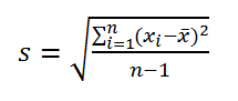
Write down a formula to calculate sample variance. Dispersion is a measure of the spread of values of a certain quantity. How closer value dispersion to zero, the closer the values are grouped to each other. When working with value selection, use the following formula to calculate variance:
- s 2 (\displaystyle s^(2)) = ∑[(x i (\displaystyle x_(i))- x̅) 2 (\displaystyle ^(2))] / (n - 1)
- s 2 (\displaystyle s^(2))– this is dispersion. Dispersion is measured in square units.
- x i (\displaystyle x_(i))– each value in the sample.
- x i (\displaystyle x_(i)) you need to subtract x̅, square it, and then add the results.
- x̅ – sample mean (sample mean).
- n – number of values in the sample.
Calculate the sample mean. It is denoted as x̅. The sample mean is calculated as a simple arithmetic mean: add up all the values in the sample, and then divide the result by the number of values in the sample.
- In our example, add the values in the sample: 15 + 17 + 23 + 7 + 9 + 13 = 84
  Now divide the result by the number of values in the sample (in our example there are 6): 84 ÷ 6 = 14.
  Sample mean x̅ = 14.
- The sample mean is the central value around which the values in the sample are distributed. If the values in the sample cluster around the sample mean, then the variance is small; otherwise the variance is large.
Subtract the sample mean from each value in the sample. Now calculate the difference x i (\displaystyle x_(i))- x̅, where x i (\displaystyle x_(i))– each value in the sample. Each result obtained indicates the degree of deviation of a particular value from the sample mean, that is, how far this value is from the sample mean.
- In our example:
  x 1 (\displaystyle x_(1))- x = 17 - 14 = 3
  x 2 (\displaystyle x_(2))- x̅ = 15 - 14 = 1
  x 3 (\displaystyle x_(3))- x = 23 - 14 = 9
  x 4 (\displaystyle x_(4))- x̅ = 7 - 14 = -7
  x 5 (\displaystyle x_(5))- x̅ = 9 - 14 = -5
  x 6 (\displaystyle x_(6))- x̅ = 13 - 14 = -1
- The correctness of the results obtained is easy to check, since their sum should be equal to zero. This is related to the determination of the average value, since negative values(distances from the average value to smaller values) are fully compensated positive values(distances from average to large values).
As noted above, the sum of the differences x i (\displaystyle x_(i))- x̅ must be equal to zero. This means that the average variance is always zero, which does not give any idea about the spread of values of a certain quantity. To solve this problem, square each difference x i (\displaystyle x_(i))- x̅. This will result in you only getting positive numbers, which when added will never give 0.
- In our example:
  (x 1 (\displaystyle x_(1))- x̅) 2 = 3 2 = 9 (\displaystyle ^(2)=3^(2)=9)
  (x 2 (\displaystyle (x_(2))- x̅) 2 = 1 2 = 1 (\displaystyle ^(2)=1^(2)=1)
  9 2 = 81
  (-7) 2 = 49
  (-5) 2 = 25
  (-1) 2 = 1
- You found the square of the difference - x̅) 2 (\displaystyle ^(2)) for each value in the sample.
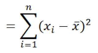
Calculate the sum of the squares of the differences. That is, find that part of the formula that is written like this: ∑[( x i (\displaystyle x_(i))- x̅) 2 (\displaystyle ^(2))]. Here the sign Σ means the sum of squared differences for each value x i (\displaystyle x_(i)) in the sample. You have already found the squared differences (x i (\displaystyle (x_(i))- x̅) 2 (\displaystyle ^(2)) for each value x i (\displaystyle x_(i)) in the sample; now just add these squares.
- In our example: 9 + 1 + 81 + 49 + 25 + 1 = 166 .
Divide the result by n - 1, where n is the number of values in the sample. Some time ago, to calculate sample variance, statisticians simply divided the result by n; in this case you will get the mean of the squared variance, which is ideal for describing the variance of a given sample. But remember that any sample is only a small part of the population of values. If you take another sample and perform the same calculations, you will get a different result. As it turns out, dividing by n - 1 (rather than just n) gives a more accurate estimate of the population variance, which is what you're interested in. Division by n – 1 has become common, so it is included in the formula for calculating sample variance.
- In our example, the sample includes 6 values, that is, n = 6.
  Sample variance = s 2 = 166 6 − 1 = (\displaystyle s^(2)=(\frac (166)(6-1))=) 33,2
The difference between variance and standard deviation. Note that the formula contains an exponent, so the dispersion is measured in square units of the value being analyzed. Sometimes such a magnitude is quite difficult to operate; in such cases, use the standard deviation, which is equal to the square root of the variance. That is why the sample variance is denoted as s 2 (\displaystyle s^(2)), A standard deviation samples - how s (\displaystyle s).
- In our example, the standard deviation of the sample is: s = √33.2 = 5.76.
Calculating Population Variance
1. Analyze some set of values. The set includes all values of the quantity under consideration. For example, if you are studying the age of residents Leningrad region, then the population includes the ages of all residents of this area. When working with a population, it is recommended to create a table and enter the population values into it. Consider the following example:
  - In a certain room there are 6 aquariums. Each aquarium contains the following number of fish:
    x 1 = 5 (\displaystyle x_(1)=5)
    x 2 = 5 (\displaystyle x_(2)=5)
    x 3 = 8 (\displaystyle x_(3)=8)
    x 4 = 12 (\displaystyle x_(4)=12)
    x 5 = 15 (\displaystyle x_(5)=15)
    x 6 = 18 (\displaystyle x_(6)=18)
2. Write down a formula to calculate the population variance. Since the totality includes all values of a certain quantity, the formula below allows us to obtain exact value population variances. To distinguish population variance from sample variance (which is only an estimate), statisticians use various variables:
  - σ 2 (\displaystyle ^(2)) = (∑(x i (\displaystyle x_(i)) - μ) 2 (\displaystyle ^(2)))/n
  - σ 2 (\displaystyle ^(2))– population dispersion (read as “sigma squared”). Dispersion is measured in square units.
  - x i (\displaystyle x_(i))– each value in its entirety.
  - Σ – sum sign. That is, from each value x i (\displaystyle x_(i)) you need to subtract μ, square it, and then add the results.
  - μ – population mean.
  - n – number of values in the population.
3. Calculate the population mean. When working with a population, its mean is denoted as μ (mu). The population mean is calculated as a simple arithmetic mean: add up all the values in the population, and then divide the result by the number of values in the population.
  - Keep in mind that averages are not always calculated as the arithmetic mean.
  - In our example, the population mean: μ = 5 + 5 + 8 + 12 + 15 + 18 6 (\displaystyle (\frac (5+5+8+12+15+18)(6))) = 10,5
4. Subtract the population mean from each value in the population. The closer the difference is to zero, the closer specific meaning to the population mean. Find the difference between each value in the population and its mean, and you will get a first idea of the distribution of values.
  - In our example:
    x 1 (\displaystyle x_(1))- μ = 5 - 10.5 = -5.5
    x 2 (\displaystyle x_(2))- μ = 5 - 10.5 = -5.5
    x 3 (\displaystyle x_(3))- μ = 8 - 10.5 = -2.5
    x 4 (\displaystyle x_(4))- μ = 12 - 10.5 = 1.5
    x 5 (\displaystyle x_(5))- μ = 15 - 10.5 = 4.5
    x 6 (\displaystyle x_(6))- μ = 18 - 10.5 = 7.5
5. Square each result obtained. The difference values will be both positive and negative; If these values are plotted on a number line, they will lie to the right and left of the population mean. This is not suitable for calculating variance, since positive and negative numbers compensate each other. So square each difference to get exclusively positive numbers.
  - In our example:
    (x i (\displaystyle x_(i)) - μ) 2 (\displaystyle ^(2)) for each population value (from i = 1 to i = 6):
    (-5,5)2 (\displaystyle ^(2)) = 30,25
    (-5,5)2 (\displaystyle ^(2)), Where x n (\displaystyle x_(n))– the last value in the population.
  - To calculate the average value of the results obtained, you need to find their sum and divide it by n:(( x 1 (\displaystyle x_(1)) - μ) 2 (\displaystyle ^(2)) + (x 2 (\displaystyle x_(2)) - μ) 2 (\displaystyle ^(2)) + ... + (x n (\displaystyle x_(n)) - μ) 2 (\displaystyle ^(2)))/n
  - Now let's write down the above explanation using variables: (∑( x i (\displaystyle x_(i)) - μ) 2 (\displaystyle ^(2))) / n and get a formula for calculating the population variance.

Let's calculate inMSEXCELsample variance and standard deviation. We will also calculate the variance of a random variable if its distribution is known.

Let's first consider dispersion, then standard deviation.

Sample variance

Sample variance (sample variance,samplevariance) characterizes the spread of values in the array relative to .

All 3 formulas are mathematically equivalent.

From the first formula it is clear that sample variance is the sum of the squared deviations of each value in the array from average, divided by sample size minus 1.

variances samples the DISP() function is used, English. the name VAR, i.e. VARiance. From version MS EXCEL 2010, it is recommended to use its analogue DISP.V(), English. the name VARS, i.e. Sample VARiance. In addition, starting from the version of MS EXCEL 2010, there is a function DISP.Г(), English. name VARP, i.e. Population VARiance, which calculates dispersion For population. The whole difference comes down to the denominator: instead of n-1 like DISP.V(), DISP.G() has just n in the denominator. Before MS EXCEL 2010, the VAR() function was used to calculate the variance of the population.

Sample variance
=QUADROTCL(Sample)/(COUNT(Sample)-1)
=(SUM(Sample)-COUNT(Sample)*AVERAGE(Sample)^2)/ (COUNT(Sample)-1)– usual formula
=SUM((Sample -AVERAGE(Sample))^2)/ (COUNT(Sample)-1) –

Sample variance is equal to 0, only if all values are equal to each other and, accordingly, equal average value. Usually, the larger the value variances, the greater the spread of values in the array.

Sample variance is a point estimate variances distribution of the random variable from which it was made sample. About construction confidence intervals when assessing variances can be read in the article.

Variance of a random variable

To calculate dispersion random variable, you need to know it.

For variances random variable X is often denoted Var(X). Dispersion equal to the square of the deviation from the mean E(X): Var(X)=E[(X-E(X)) 2 ]

dispersion calculated by the formula:

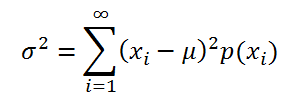
where x i is the value that a random variable can take, and μ is the average value (), p(x) is the probability that the random variable will take the value x.

If a random variable has , then dispersion calculated by the formula:

Dimension variances corresponds to the square of the unit of measurement of the original values. For example, if the values in the sample represent part weight measurements (in kg), then the variance dimension would be kg 2 . This can be difficult to interpret, so to characterize the spread of values, a value equal to the square root of variances – standard deviation.

Some properties variances:

Var(X+a)=Var(X), where X is a random variable and a is a constant.

Var(aХ)=a 2 Var(X)

Var(X)=E[(X-E(X)) 2 ]=E=E(X 2)-E(2*X*E(X))+(E(X)) 2 =E(X 2)- 2*E(X)*E(X)+(E(X)) 2 =E(X 2)-(E(X)) 2

This dispersion property is used in article about linear regression.

Var(X+Y)=Var(X) + Var(Y) + 2*Cov(X;Y), where X and Y are random variables, Cov(X;Y) is the covariance of these random variables.

If random variables are independent, then they covariance is equal to 0, and therefore Var(X+Y)=Var(X)+Var(Y). This property of dispersion is used in derivation.

Let us show that for independent quantities Var(X-Y)=Var(X+Y). Indeed, Var(X-Y)= Var(X-Y)= Var(X+(-Y))= Var(X)+Var(-Y)= Var(X)+Var(-Y)= Var( X)+(-1) 2 Var(Y)= Var(X)+Var(Y)= Var(X+Y). This dispersion property is used to construct .

Sample standard deviation

Sample standard deviation is a measure of how widely scattered the values in a sample are relative to their .

A-priory, standard deviation equal to the square root of variances:

Standard deviation does not take into account the magnitude of the values in sample, but only the degree of dispersion of values around them average. To illustrate this, let's give an example.

Let's calculate the standard deviation for 2 samples: (1; 5; 9) and (1001; 1005; 1009). In both cases, s=4. It is obvious that the ratio of the standard deviation to the array values differs significantly between samples. For such cases it is used The coefficient of variation(Coefficient of Variation, CV) - ratio Standard Deviation to the average arithmetic, expressed as a percentage.

In MS EXCEL 2007 and earlier versions for calculation Sample standard deviation the function =STDEVAL() is used, English. name STDEV, i.e. STandard DEViation. From the version of MS EXCEL 2010, it is recommended to use its analogue =STDEV.B() , English. name STDEV.S, i.e. Sample STandard DEViation.

In addition, starting from the version of MS EXCEL 2010, there is a function STANDARDEV.G(), English. name STDEV.P, i.e. Population STandard DEViation, which calculates standard deviation For population. The whole difference comes down to the denominator: instead of n-1 as in STANDARDEV.V(), STANDARDEVAL.G() has just n in the denominator.

Standard deviation can also be calculated directly using the formulas below (see example file)
=ROOT(QUADROTCL(Sample)/(COUNT(Sample)-1))
=ROOT((SUM(Sample)-COUNT(Sample)*AVERAGE(Sample)^2)/(COUNT(Sample)-1))

Other measures of scatter

The SQUADROTCL() function calculates with a sum of squared deviations of values from their average. This function will return the same result as the formula =DISP.G( Sample)*CHECK( Sample) , Where Sample- a reference to a range containing an array of sample values (). Calculations in the QUADROCL() function are made according to the formula:

The SROTCL() function is also a measure of the spread of a data set. The function SROTCL() calculates the average of the absolute values of deviations of values from average. This function will return the same result as the formula =SUMPRODUCT(ABS(Sample-AVERAGE(Sample)))/COUNT(Sample), Where Sample- a link to a range containing an array of sample values.

Calculations in the function SROTCL () are made according to the formula:

Conversely, if is a non-negative a.e. function such that , then there is an absolutely continuous probability measure on such that it is its density.

Replacing the measure in the Lebesgue integral:

where is any Borel function that is integrable with respect to the probability measure.

Dispersion, types and properties of dispersion The concept of dispersion

Dispersion in statistics is found as the standard deviation of the individual values of the characteristic squared from the arithmetic mean. Depending on the initial data, it is determined using the simple and weighted variance formulas:

1. Simple variance(for ungrouped data) is calculated using the formula:

2. Weighted variance (for variation series):

where n is frequency (repeatability of factor X)

An example of finding variance

This page describes a standard example of finding variance, you can also look at other problems for finding it

Example 1. Determination of group, group average, intergroup and total variance

Example 2. Finding the variance and coefficient of variation in a grouping table

Example 3. Finding variance in a discrete series

Example 4. The following data is available for a group of 20 correspondence students. It is necessary to construct an interval series of the distribution of the characteristic, calculate the average value of the characteristic and study its dispersion

Let's build an interval grouping. Let's determine the range of the interval using the formula:

where X max is the maximum value of the grouping characteristic; X min – minimum value of the grouping characteristic; n – number of intervals:

We accept n=5. The step is: h = (192 - 159)/ 5 = 6.6

Let's create an interval grouping

For further calculations, we will build an auxiliary table:

X"i – the middle of the interval. (for example, the middle of the interval 159 – 165.6 = 162.3)

We determine the average height of students using the weighted arithmetic average formula:

Let's determine the variance using the formula:

The formula can be transformed like this:

From this formula it follows that variance is equal to the difference between the average of the squares of the options and the square and the average.

where i is the value of the interval; A is a conventional zero, for which it is convenient to use the middle of the interval with the highest frequency; m1 is the square of the first order moment; m2 - moment of second order

Substituting q = 1- p into this dispersion formula, we get:

Types of variance

Thus, within-group variance measures variation of a trait within a group and is determined by the formula:

where xi is the group average; ni is the number of units in the group.

For example, intragroup variances that need to be determined in the task of studying the influence of workers’ qualifications on the level of labor productivity in a workshop show variations in output in each group caused by all possible factors (technical condition of equipment, availability of tools and materials, age of workers, labor intensity, etc. .), except for differences in qualification category (within a group all workers have the same qualifications).

The average of within-group variances reflects random variation, that is, that part of the variation that occurred under the influence of all other factors, with the exception of the grouping factor. It is calculated using the formula:

Intergroup variance characterizes the systematic variation of the resulting characteristic, which is due to the influence of the factor-attribute that forms the basis of the group. It is equal to the mean square of the deviations of the group means from the overall mean. Intergroup variance is calculated using the formula:

However, this characteristic alone is not enough to study a random variable. Let's imagine two shooters shooting at a target. One shoots accurately and hits close to the center, while the other... is just having fun and doesn’t even aim. But what's funny is that he average the result will be exactly the same as the first shooter! This situation is conventionally illustrated by the following random variables:

The “sniper” mathematical expectation is equal to , however, for the “interesting person”: – it is also zero!

Thus, there is a need to quantify how far scattered bullets (random variable values) relative to the center of the target (mathematical expectation). well and scattering translated from Latin is no other way than dispersion .

Let's see how this numerical characteristic is determined using one of the examples from the 1st part of the lesson:

There we found a disappointing mathematical expectation of this game, and now we have to calculate its variance, which denoted by through .

Let's find out how far the wins/losses are “scattered” relative to the average value. Obviously, for this we need to calculate differences between random variable values and her mathematical expectation:

–5 – (–0,5) = –4,5
2,5 – (–0,5) = 3
10 – (–0,5) = 10,5

Now it seems that you need to sum up the results, but this way is not suitable - for the reason that fluctuations to the left will cancel each other out with fluctuations to the right. So, for example, an “amateur” shooter (example above) the differences will be , and when added they will give zero, so we will not get any estimate of the dispersion of his shooting.

To get around this problem you can consider modules differences, but for technical reasons the approach has taken root when they are squared. It is more convenient to formulate the solution in a table:

And here it begs to calculate weighted average the value of the squared deviations. What is it? It's theirs expected value, which is a measure of scattering:

– definition variances. From the definition it is immediately clear that variance cannot be negative– take note for practice!

Let's remember how to find the expected value. Multiply the squared differences by the corresponding probabilities (Table continuation):
– figuratively speaking, this is “traction force”,
and summarize the results:

Don't you think that compared to the winnings, the result turned out to be too big? That's right - we squared it, and to return to the dimension of our game, we need to extract Square root. This quantity is called standard deviation and is denoted by the Greek letter “sigma”:

This value is sometimes called standard deviation .

What is its meaning? If we deviate from the mathematical expectation to the left and right by the standard deviation:

– then the most probable values of the random variable will be “concentrated” on this interval. What we actually observe:

However, it so happens that when analyzing scattering one almost always operates with the concept of dispersion. Let's figure out what it means in relation to games. If in the case of arrows we are talking about the “accuracy” of hits relative to the center of the target, then here dispersion characterizes two things:

Firstly, it is obvious that as the bets increase, the dispersion also increases. So, for example, if we increase by 10 times, then the mathematical expectation will increase by 10 times, and the variance will increase by 100 times (since this is a quadratic quantity). But note that the rules of the game themselves have not changed! Only the rates have changed, roughly speaking, before we bet 10 rubles, now it’s 100.

Second, more interesting point is that variance characterizes the style of play. Mentally fix the game bets at some certain level, and let's see what's what:

A low variance game is a cautious game. The player tends to choose the most reliable schemes, where he does not lose/win too much at one time. For example, the red/black system in roulette (see example 4 of the article Random variables) .

High variance game. She is often called dispersive game. This is an adventurous or aggressive style of play, where the player chooses “adrenaline” schemes. Let's at least remember "Martingale", in which the amounts at stake are orders of magnitude greater than the “quiet” game of the previous point.

The situation in poker is indicative: there are so-called tight players who tend to be cautious and “shaky” over their gaming means (bankroll). Not surprisingly, their bankroll does not fluctuate significantly (low variance). On the contrary, if a player has high variance, then he is an aggressor. He often takes risks, makes large bets and can either break a huge bank or lose to smithereens.

The same thing happens in Forex, and so on - there are plenty of examples.

Moreover, in all cases it does not matter whether the game is played for pennies or thousands of dollars. Every level has its low- and high-dispersion players. Well, as we remember, the average winning is “responsible” expected value.

You probably noticed that finding variance is a long and painstaking process. But mathematics is generous:

Formula for finding variance

This formula is derived directly from the definition of variance, and we immediately put it into use. I’ll copy the sign with our game above:

and the found mathematical expectation.

Let's calculate the variance in the second way. First, let's find the mathematical expectation - the square of the random variable. By determination of mathematical expectation:

IN in this case:

Thus, according to the formula:

As they say, feel the difference. And in practice, of course, it is better to use the formula (unless the condition requires otherwise).

We master the technique of solving and designing:

Example 6

Find its mathematical expectation, variance and standard deviation.

This task is found everywhere, and, as a rule, goes without meaningful meaning.
You can imagine several light bulbs with numbers that light up in a madhouse with certain probabilities :)

Solution: It is convenient to summarize the basic calculations in a table. First, we write the initial data in the top two lines. Then we calculate the products, then and finally the sums in the right column:

Actually, almost everything is ready. The third line shows a ready-made mathematical expectation: .

We calculate the variance using the formula:

And finally, the standard deviation:
– Personally, I usually round to 2 decimal places.

All calculations can be carried out on a calculator, or even better – in Excel:

It's hard to go wrong here :)

Answer:

Those who wish can simplify their life even more and take advantage of my calculator (demo), which will not only instantly solve this problem, but also build thematic graphics (we'll get there soon). The program can be download from the library– if you have downloaded at least one educational material, or get another way. Thanks for supporting the project!

A couple of tasks to solve on your own:

Example 7

Calculate the variance of the random variable in the previous example by definition.

AND similar example:

Example 8

A discrete random variable is specified by its distribution law:

Yes, random variable values can be quite large (example from real work) , and here, if possible, use Excel. As, by the way, in Example 7 - it’s faster, more reliable and more enjoyable.

Solutions and answers at the bottom of the page.

At the end of the 2nd part of the lesson, we will look at one more typical task, one might even say, a small rebus:

Example 9

A discrete random variable can take only two values: and , and . The probability, mathematical expectation and variance are known.

Solution: Let's start with an unknown probability. Since a random variable can take only two values, the sum of the probabilities of the corresponding events is:

and since , then .

All that remains is to find..., it's easy to say :) But oh well, here we go. By definition of mathematical expectation:
– substitute known quantities:

– and nothing more can be squeezed out of this equation, except that you can rewrite it in the usual direction:

or:

ABOUT further actions, I think you can guess. Let's compose and solve the system:

Decimals- this, of course, is a complete disgrace; multiply both equations by 10:

and divide by 2:

That's better. From the 1st equation we express:
(this is the easier way)– substitute into the 2nd equation:

We are building squared and make simplifications:

Multiply by:

The result was quadratic equation, we find its discriminant:
- Great!

and we get two solutions:

1) if , That ;

2) if , That .

The condition is satisfied by the first pair of values. With a high probability everything is correct, but, nevertheless, let’s write down the distribution law:

and perform a check, namely, find the expectation: