Taylor series expansion of the square root. Expansion of a function into a Taylor, Maclaurin, Laurent series

Among functional series, the most important place is occupied by power series.

A power series is a series

whose members are power functions, arranged in increasing integer non-negative powers x, A c0 , c 1 , c 2 , c n - constant values. Numbers c1 , c 2 , c n - coefficients of the series terms, c0 - free member. Members power series defined on the entire number line.

Let's get acquainted with the concept areas of convergence of the power series. This is a set of variable values x, for which the series converges. Power series have a fairly simple convergence region. For real variable values x the convergence region consists either of one point, or is a certain interval (convergence interval), or coincides with the entire axis Ox .

When substituting the values ​​into the power series x= 0 will result in a number series

c0 +0+0+...+0+... ,

which converges.

Therefore, when x= 0 any power series converges and, therefore, its area of ​​convergence cannot be the empty set. The structure of the region of convergence of all power series is the same. It can be established using the following theorem.

Theorem 1 (Abel's theorem). If a power series converges at some value x = x 0 , different from zero, then it converges, and, moreover, absolutely, for all values |x| < |x 0 | . Please note: both the starting value “X is zero” and any value of “X” that is compared with the starting value are taken modulo - without taking into account the sign.

Consequence. If power series diverges at some value x = x 1 , then it diverges for all values |x| > |x 1 | .

As we have already found out earlier, any power series converges at the value x= 0. There are power series that converge only when x= 0 and diverge for other values X. Excluding this case from consideration, we assume that the power series converges at some value x = x 0 , different from zero. Then, according to Abel's theorem, it converges at all points of the interval ]-| x0 |, |x 0 |[ (an interval whose left and right boundaries are the x values ​​at which the power series converges, taken with a minus sign and a plus sign, respectively), symmetrical with respect to the origin.

If the power series diverges at a certain value x = x 1 , then, based on a corollary to Abel’s theorem, it diverges at all points outside the segment [-| x1 |, |x 1 |] . It follows that for any power series there is an interval symmetric with respect to the origin, called convergence interval , at each point of which the series converges, at the boundaries it can converge, or it can diverge, and not necessarily at the same time, and outside the segment the series diverges. Number R is called the radius of convergence of the power series.

In special cases convergence interval of power series can degenerate to a point (then the series converges only when x= 0 and it is considered that R= 0) or represent the entire number line (then the series converges at all points of the number line and it is assumed that ).

Thus, determining the region of convergence of a power series consists in determining its convergence radius R and studying the convergence of the series at the boundaries of the convergence interval (at ).

Theorem 2. If all the coefficients of a power series, starting from a certain one, are different from zero, then its radius of convergence is equal to the limit at the ratio of the absolute values ​​of the coefficients of the common following members of the series, i.e.

Example 1. Find the region of convergence of the power series

Solution. Here

Using formula (28), we find the radius of convergence of this series:

Let us study the convergence of the series at the ends of the convergence interval. Example 13 shows that this series converges at x= 1 and diverges at x= -1. Consequently, the region of convergence is the half-interval.

Example 2. Find the region of convergence of the power series

Solution. The coefficients of the series are positive, and

Let us find the limit of this ratio, i.e. radius of convergence of the power series:

Let us study the convergence of the series at the ends of the interval. Substitution of values x= -1/5 and x= 1/5 in this row gives:

The first of these series converges (see Example 5). But then, by virtue of the theorem in the “Absolute convergence” section, the second series also converges, and the region of its convergence is the segment

Example 3. Find the region of convergence of the power series

Solution. Here

Using formula (28) we find the radius of convergence of the series:

Let us study the convergence of the series for values ​​of . Substituting them in this series, we respectively obtain

Both series diverge because the necessary condition for convergence is not satisfied (their common terms do not tend to zero at ). So, at both ends of the convergence interval, this series diverges, and the region of its convergence is the interval.

Example 5. Find the region of convergence of the power series

Solution. We find the relation where , and :

According to formula (28), the radius of convergence of this series

,

that is, the series converges only when x= 0 and diverges for other values X.

Examples show that at the ends of the convergence interval the series behave differently. In example 1, at one end of the convergence interval the series converges, and at the other, it diverges; in example 2, it converges at both ends; in example 3, it diverges at both ends.

The formula for the radius of convergence of a power series is obtained under the assumption that all coefficients of the series terms, starting from a certain point, are different from zero. Therefore, the use of formula (28) is permissible only in these cases. If this condition is violated, then the radius of convergence of the power series should be sought using d'Alembert's sign, or, by replacing the variable, transforming the series to a form in which the specified condition is satisfied.

Example 6. Find the interval of convergence of the power series

Solution. This series does not contain terms with odd degrees X. Therefore, we transform the series, setting . Then we get the series

to find the radius of convergence of which we can apply formula (28). Since , a , then the radius of convergence of this series

From the equality we obtain , therefore, this series converges on the interval .

Sum of power series. Differentiation and integration of power series

Let for the power series

radius of convergence R> 0, i.e. this series converges on the interval .

Then each value X from the convergence interval corresponds to a certain sum of the series. Therefore, the sum of the power series is a function of X on the convergence interval. Denoting it by f(x), we can write the equality

understanding it in the sense that the sum of the series at each point X from the convergence interval is equal to the value of the function f(x) at this point. In the same sense, we will say that the power series (29) converges to the function f(x) on the convergence interval.

Outside the convergence interval, equality (30) makes no sense.

Example 7. Find the sum of the power series

Solution. This is a geometric series for which a= 1, a q= x. Therefore, its sum is a function . A series converges if , and is its convergence interval. Therefore equality

is valid only for values, although the function defined for all values X, except X= 1.

It can be proven that the sum of the power series f(x) is continuous and differentiable on any interval within the convergence interval, in particular at any point in the convergence interval of the series.

Let us present theorems on term-by-term differentiation and integration of power series.

Theorem 1. Power series (30) in the interval of its convergence can be differentiated term by term an unlimited number of times, and the resulting power series have the same radius of convergence as the original series, and their sums are respectively equal to .

Theorem 2. Power series (30) can be integrated term by term an unlimited number of times in the range from 0 to X, if , and the resulting power series have the same radius of convergence as the original series, and their sums are correspondingly equal

Expansion of functions into power series

Let the function be given f(x), which needs to be expanded into a power series, i.e. represent in the form (30):

The task is to determine the coefficients row (30). To do this, differentiating equality (30) term by term, we consistently find:

……………………………………………….. (31)

Assuming in equalities (30) and (31) X= 0, we find

Substituting the found expressions into equality (30), we obtain

(32)

Let us find the Maclaurin series expansion of some elementary functions.

Example 8. Expand the function in a Maclaurin series

Solution. The derivatives of this function coincide with the function itself:

Therefore, when X= 0 we have

Substituting these values ​​into formula (32), we obtain the desired expansion:

(33)

This series converges on the entire number line (its radius of convergence).

Expansion of a function into a Taylor, Maclaurin and Laurent series on a site for training practical skills. This series expansion of a function allows mathematicians to estimate the approximate value of the function at some point in its domain of definition. It is much easier to calculate such a function value compared to using the Bredis table, which is so irrelevant in this century computer technology. Expanding a function into a Taylor series means calculating the coefficients before linear functions this series and write it down in correct form. Students confuse these two series, not understanding what is general case, and what is a special case of the second. Let us remind you once and for all that the Maclaurin series is a special case of the Taylor series, that is, this is the Taylor series, but at the point x = 0. All brief entries for the expansion of well-known functions, such as e^x, Sin(x), Cos(x) and others, these are Taylor series expansions, but at point 0 for the argument. For functions of a complex argument, the Laurent series is the most common problem in TFCT, since it represents a two-sided infinite series. It is the sum of two series. We suggest you look at an example of decomposition directly on the website; this is very easy to do by clicking on “Example” with any number, and then the “Solution” button. It is precisely this expansion of a function into a series that is associated with a majorizing series that limits the original function in a certain region along the ordinate axis if the variable belongs to the abscissa region. Vector analysis is compared to another interesting discipline in mathematics. Since each term needs to be examined, the process requires quite a lot of time. Any Taylor series can be associated with a Maclaurin series by replacing x0 with zero, but for a Maclaurin series it is sometimes not obvious to represent the Taylor series in reverse. As if this is not required to be done in its pure form, it is interesting for general self-development. Every Laurent series corresponds to a two-sided infinite power series in integers powers z-a, in other words, a series of the same Taylor type, but slightly different in the calculation of coefficients. We’ll talk about the region of convergence of the Laurent series a little later, after several theoretical calculations. As in the last century, a step-by-step expansion of a function into a series can hardly be achieved simply by bringing the terms to a common denominator, since the functions in the denominators are nonlinear. An approximate calculation of the functional value is required by the formulation of problems. Think about the fact that when the argument of a Taylor series is a linear variable, then the expansion occurs in several steps, but the picture is completely different when the argument of the function being expanded is a complex or nonlinear function, then the process of representing such a function in a power series is obvious, since, in this way Thus, it is easy to calculate, albeit an approximate value, at any point in the definition region, with a minimum error that has little effect on further calculations. This also applies to the Maclaurin series. when it is necessary to calculate the function at the zero point. However, the Laurent series itself is represented here by an expansion on the plane with imaginary units. It will also not be without success correct solution tasks during the overall process. This approach is not known in mathematics, but it objectively exists. As a result, you can come to the conclusion of the so-called pointwise subsets, and in the expansion of a function in a series you need to use methods known for this process, such as the application of the theory of derivatives. Once again we are convinced that the teacher was right, who made his assumptions about the results of post-computational calculations. Let's note that the Taylor series, obtained according to all the canons of mathematics, exists and is defined on the entire numerical axis, however, dear users of the site service, do not forget the type of the original function, because it may turn out that initially it is necessary to establish the domain of definition of the function, that is, write and exclude from further consideration those points at which the function is not defined in the region real numbers. So to speak, this will show your efficiency in solving the problem. The construction of a Maclaurin series with a zero argument value will not be an exception to what has been said. The process of finding the domain of definition of a function has not been canceled, and you must approach this mathematical operation with all seriousness. In the case of a Laurent series containing the main part, the parameter “a” will be called an isolated singular point, and the Laurent series will be expanded in a ring - this is the intersection of the areas of convergence of its parts, hence the corresponding theorem will follow. But not everything is as complicated as it might seem at first glance to an inexperienced student. Having studied the Taylor series, you can easily understand the Laurent series - a generalized case for expanding the space of numbers. Any series expansion of a function can be performed only at a point in the domain of definition of the function. Properties of functions such as periodicity or infinite differentiability should be taken into account. We also suggest that you use the table of ready-made Taylor series expansions of elementary functions, since one function can be represented by up to dozens of different power series, as can be seen from using our online calculator. Online series Maclaurin is easy to determine if you use unique service site, you just need to enter the correct written function and you will receive the presented answer in a matter of seconds, it will be guaranteed to be accurate and in a standard written form. You can copy the result directly into a clean copy for submission to the teacher. It would be correct to first determine the analyticity of the function in question in rings, and then unambiguously state that it is expandable in a Laurent series in all such rings. It is important not to lose sight of the contents negative powers members of the Laurent series. Focus on this as much as possible. Make good use of Laurent's theorem on the expansion of a function in integer powers.

In the theory of functional series, the central place is occupied by the section devoted to the expansion of a function into a series.

Thus, the task is set: for a given function we need to find such a power series

which converged on a certain interval and its sum was equal to
, those.

= ..

This task is called the problem of expanding a function into a power series.

A necessary condition for the decomposability of a function in a power series is its differentiability an infinite number of times - this follows from the properties of convergent power series. This condition is satisfied, as a rule, for elementary functions in their domain of definition.

So let's assume that the function
has derivatives of any order. Is it possible to expand it into a power series? If so, how can we find this series? The second part of the problem is easier to solve, so let’s start with it.

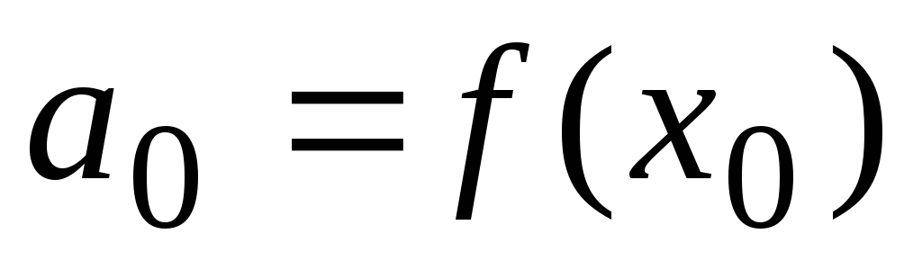
Let us assume that the function
can be represented as the sum of a power series converging in the interval containing the point X 0 :

= .. (*)

Where A 0 ,A 1 ,A 2 ,...,A P ,... – unknown (yet) coefficients.

Let us put in equality (*) the value x = x 0 , then we get

.

Let us differentiate the power series (*) term by term

= ..

and believing here x = x 0 , we get

.

With the next differentiation we obtain the series

= ..

believing x = x 0 , we get
, where
.

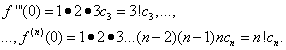
After P-multiple differentiation we get

Assuming in the last equality x = x 0 , we get
, where

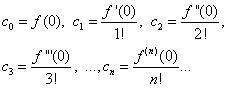
So, the coefficients are found

,
,
, …,
,….,

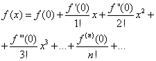
substituting which into the series (*), we get

The resulting series is called next to Taylor for function
.

Thus, we have established that if the function can be expanded into a power series in powers (x - x 0 ), then this expansion is unique and the resulting series is necessarily a Taylor series.

Note that the Taylor series can be obtained for any function that has derivatives of any order at the point x = x 0 . But this does not mean that an equal sign can be placed between the function and the resulting series, i.e. that the sum of the series is equal to the original function. Firstly, such an equality can only make sense in the region of convergence, and the Taylor series obtained for the function may diverge, and secondly, if the Taylor series converges, then its sum may not coincide with the original function.

3.2. Sufficient conditions for the decomposability of a function in a Taylor series

Let us formulate a statement with the help of which the task will be solved.

If the function
in some neighborhood of point x 0 has derivatives up to (n+ 1) of order inclusive, then in this neighborhood we haveformula Taylor

WhereR n (X)-the remainder term of the Taylor formula – has the form (Lagrange form)

Where dotξ lies between x and x 0 .

Note that there is a difference between the Taylor series and the Taylor formula: the Taylor formula is a finite sum, i.e. P - fixed number.

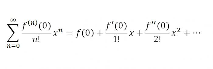
Recall that the sum of the series S(x) can be defined as the limit of a functional sequence of partial sums S P (x) at some interval X:

.

According to this, to expand a function into a Taylor series means to find a series such that for any XX

Let us write Taylor's formula in the form where

notice, that
defines the error we get, replace the function f(x) polynomial S n (x).

If
, That
,those. the function is expanded into a Taylor series. Vice versa, if
, That
.

Thus we proved criterion for the decomposability of a function in a Taylor series.

In order for the functionf(x) expands into a Taylor series, it is necessary and sufficient that on this interval
, WhereR n (x) is the remainder term of the Taylor series.

Using the formulated criterion, one can obtain sufficientconditions for the decomposability of a function in a Taylor series.

If insome neighborhood of point x 0 the absolute values ​​of all derivatives of the function are limited to the same number M≥ 0, i.e.

, To in this neighborhood the function expands into a Taylor series.

From the above it follows algorithmfunction expansion f(x) in the Taylor series in the vicinity of a point X 0 :

1. Finding derivatives of functions f(x):

f(x), f’(x), f”(x), f’”(x), f (n) (x),…

2. Calculate the value of the function and the values ​​of its derivatives at the point X 0

f(x 0 ), f’(x 0 ), f”(x 0 ), f’”(x 0 ), f (n) (x 0 ),…

3. We formally write the Taylor series and find the region of convergence of the resulting power series.

4. We check the fulfillment of sufficient conditions, i.e. we establish for which X from the convergence region, remainder term R n (x) tends to zero as
or
.

The expansion of functions into a Taylor series using this algorithm is called expansion of a function into a Taylor series by definition or direct decomposition.

"Find the Maclaurin series expansion of the function f(x)"- this is exactly what the task in higher mathematics sounds like, which some students can do, while others cannot cope with the examples. There are several ways to expand a series in powers; here we will give a technique for expanding functions into a Maclaurin series. When developing a function in a series, you need to be good at calculating derivatives.

Example 4.7 Expand a function in powers of x

Calculations: We perform the expansion of the function according to the Maclaurin formula. First, let's expand the denominator of the function into a series

Finally, multiply the expansion by the numerator.
The first term is the value of the function at zero f (0) = 1/3.
Let's find the derivatives of the function of the first and higher orders f (x) and the value of these derivatives at the point x=0




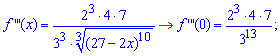
Next, based on the pattern of changes in the value of derivatives at 0, we write the formula for the nth derivative

So, we represent the denominator in the form of an expansion in the Maclaurin series

We multiply by the numerator and obtain the desired expansion of the function in a series in powers of x

As you can see, there is nothing complicated here.
All key points are based on the ability to calculate derivatives and quickly generalize the value of the higher order derivative at zero. The following examples will help you learn how to quickly arrange a function in a row.

Example 4.10 Find the Maclaurin series expansion of the function

Calculations: As you may have guessed, we will put the cosine in the numerator in a series. To do this, you can use formulas for infinitesimal quantities, or derive the expansion of the cosine through derivatives. As a result, we arrive at the following series in powers of x

As you can see, we have a minimum of calculations and a compact representation of the series expansion.

Example 4.16 Expand a function in powers of x:
7/(12-x-x^2)
Calculations: In this kind of examples, it is necessary to expand the fraction through the sum of simple fractions.
We will not show how to do this now, but with the help of indefinite coefficients we will arrive at the sum of fractions.
Next we write the denominators in exponential form

It remains to expand the terms using the Maclaurin formula. Summarizing the terms at equal degrees"x" we compose a formula for the general term of the series expansion of a function



The last part of the transition to the series at the beginning is difficult to implement, since it is difficult to combine the formulas for paired and unpaired indices (degrees), but with practice you will get better at it.

Example 4.18 Find the Maclaurin series expansion of the function

Calculations: Let's find the derivative of this function:

Let's expand the function into a series using one of McLaren's formulas:

We sum the series term by term based on the fact that both are absolutely identical. Having integrated the entire series term by term, we obtain the expansion of the function into a series in powers of x

There is a transition between the last two lines of the expansion which will take a lot of your time at the beginning. Generalizing a series formula isn't easy for everyone, so don't worry about not being able to get a nice, compact formula.

Example 4.28 Find the Maclaurin series expansion of the function:

Let's write the logarithm as follows

Using Maclaurin’s formula, we expand the logarithm function in a series in powers of x

The final convolution is complex at first glance, but when alternating signs you will always get something similar. Input lesson on the topic of scheduling functions in a row is completed. Others no less interesting schemes decompositions will be discussed in detail in the following materials.

For students higher mathematics it should be known that the sum of a certain power series belonging to the interval of convergence of the series given to us turns out to be a continuous and unlimited number of times differentiated function. The question arises: is it possible to say that a given arbitrary function f(x) is the sum of a certain power series? That is, under what conditions can the function f(x) be depicted? power series? The importance of this question lies in the fact that it is possible to approximately replace the function f(x) with the sum of the first few terms of a power series, that is, a polynomial. This replacement of a function with a rather simple expression - a polynomial - is also convenient when solving certain problems, namely: when solving integrals, when calculating, etc.

It has been proven that for a certain function f(x), in which it is possible to calculate derivatives up to the (n+1)th order, including the last, in the neighborhood of (α - R; x 0 + R) some point x = α, it is true that formula:

This formula is named after the famous scientist Brooke Taylor. The series that is obtained from the previous one is called the Maclaurin series:

The rule that makes it possible to perform an expansion in a Maclaurin series:

1. Determine derivatives of the first, second, third... orders.
2. Calculate what the derivatives at x=0 are equal to.
3. Write down the Maclaurin series for this function, and then determine the interval of its convergence.
4. Determine the interval (-R;R), where the remainder of the Maclaurin formula

R n (x) -> 0 at n -> infinity. If one exists, the function f(x) in it must coincide with the sum of the Maclaurin series.

Let us now consider the Maclaurin series for individual functions.

1. So, the first one will be f(x) = e x. Of course, by its characteristics, such a function has derivatives of very different orders, and f (k) (x) = e x , where k equals all. Substitute x = 0. We get f (k) (0) = e 0 =1, k = 1,2... Based on the above, the series e x will look like this:

2. Maclaurin series for the function f(x) = sin x. Let us immediately clarify that the function for all unknowns will have derivatives, in addition, f "(x) = cos x = sin(x+n/2), f "" (x) = -sin x = sin(x +2*n/2)..., f (k) (x) = sin(x+k*n/2), where k equals any natural number. That is, having made simple calculations, we can come to the conclusion that the series for f(x) = sin x will be of the following form:

3. Now let's try to consider the function f(x) = cos x. For all unknowns it has derivatives of arbitrary order, and |f (k) (x)| = |cos(x+k*n/2)|<=1, k=1,2... Снова-таки, произведя определенные расчеты, получим, что ряд для f(х) = cos х будет выглядеть так:

So, we have listed the most important functions that can be expanded in a Maclaurin series, but they are supplemented by Taylor series for some functions. Now we will list them. It is also worth noting that Taylor and Maclaurin series are an important part of practical work on solving series in higher mathematics. So, Taylor series.

1. The first will be the series for the function f(x) = ln(1+x). As in the previous examples, for the given f(x) = ln(1+x) we can add the series using the general form of the Maclaurin series. however, for this function the Maclaurin series can be obtained much more simply. Having integrated a certain geometric series, we obtain a series for f(x) = ln(1+x) of such a sample:

2. And the second, which will be final in our article, will be the series for f(x) = arctan x. For x belonging to the interval [-1;1] the expansion is valid:

That's all. This article examined the most used Taylor and Maclaurin series in higher mathematics, in particular in economics and technical universities.